Install discourse from Github.
# install devtools if needed
if (!requireNamespace("devtools")) {install.packages("devtools")}

# install from GitHub
devtools::install_github("sebastian-lortz/discourse")
Load the discourse package.
ANOVA Module
As part of the Open Science Collaboration’s large‐scale effort to estimate the replicability of psychological findings (Open-Science-Collaboration, 2015), many original datasets remain unavailable. In the study by Reynolds and Besner (2008) on contextual effects in reading aloud, participants’ response times to exception words and nonwords were measured under predictable switch and stay sequences to probe dynamic pathway control in skilled reading [https://osf.io/hasfu/]. In the following steps, I applied DISCOURSE to demonstrate how it’s ANOVA module can generate a fully synthetic dataset matching the reported summary estimates.
I began by extracting the relevant parameters from the article.
N = 16
levels = c(2,2)
target_group_means <- c(543, 536, 614, 618)
factor_type <- c("within", "within")
formula <- "outcome ~ Factor1 * Factor2 + Error(ID / (Factor1 * Factor2))"
integer <- FALSE
Factor2 and Interaction effects are reported as F < 1, thus, I set arbitrary values
I then computed a plausible response time range [L,U] from the pooled
MSE = 3070 using
L <- min(target_group_means) - floor(3 * sqrt(3070))
U <- max(target_group_means) + ceiling(3 * sqrt(3070))
L
#> [1] 370
U
#> [1] 785
range <- c(370,785)
Next, I ran the ANOVA module with a small max_step to
avoid early convergence given the coarse target precision and otherwise
default hyperparameters.
result.aov <- optim_aov(N = N,
                        levels = levels,
                        target_group_means = target_group_means,
                        target_f_list = target_f_vec,
                        factor_type = factor_type,
                        range = range,
                        formula = formula,
                        integer = integer,
                        max_step = .1,
                        tolerance = 1e-8,
                        max_iter = 1e3,
                        init_temp = 1,
                        cooling_rate = NULL)
#>   |                                                                              |                                                                      |   0%  |                                                                              |=                                                                     |   1%  |                                                                              |=                                                                     |   2%  |                                                                              |==                                                                    |   3%  |                                                                              |===                                                                   |   4%  |                                                                              |====                                                                  |   5%  |                                                                              |====                                                                  |   6%  |                                                                              |=====                                                                 |   7%  |                                                                              |======                                                                |   8%  |                                                                              |======                                                                |   9%  |                                                                              |=======                                                               |  10%  |                                                                              |========                                                              |  11%  |                                                                              |========                                                              |  12%  |                                                                              |=========                                                             |  13%  |                                                                              |==========                                                            |  14%  |                                                                              |==========                                                            |  15%  |                                                                              |===========                                                           |  16%  |                                                                              |============                                                          |  17%  |                                                                              |=============                                                         |  18%  |                                                                              |=============                                                         |  19%
The optimization converged exactly. Inspecting
summary(result.aov)
#> DISCOURSE Object Summary
#> -------------------------------------------------
#>
#> Achieved Loss of Optimization:  0
#>
#> RMSE of F statistics:  0
#>
#> Factorial Model:
#> outcome ~ Factor1 * Factor2 + Error(ID/(Factor1 * Factor2))
#>
#> Group Means:
#> [1] 543 536 614 618
confirms that the simulated data reproduce the published cell means and F-statistics. I then visualized the error trajectory
plot_error(result.aov)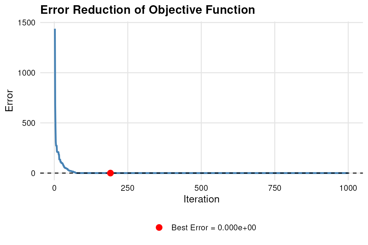
and illustrated the estimated versus target effects with
plot_summary(result.aov, standardised = FALSE)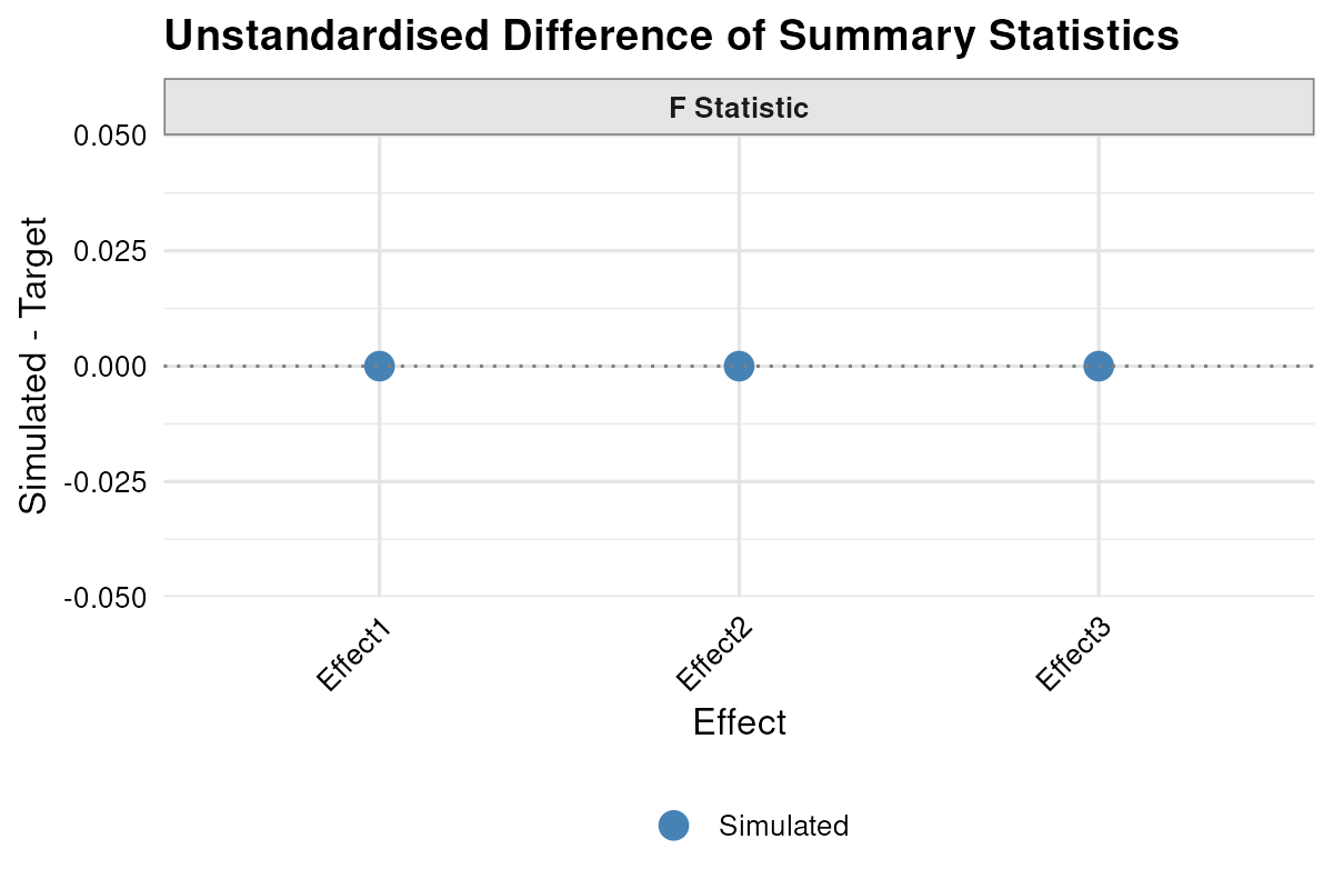 . Finally, I saved the RMSE and relevant statistics,
get_rmse(result.aov)
#> $rmse_F
#> [1] 0
get_stats(result.aov)
#> $model
#> Anova Table (Type 3 tests)
#>
#> Response: outcome
#>                 num Df den Df    MSE       F     ges    Pr(>F)
#> Factor1              1     15 3072.2 30.4789 0.44810 5.872e-05 ***
#> Factor2              1     15 1186.0  0.0304 0.00031    0.8640
#> Factor1:Factor2      1     15 2166.8  0.2234 0.00418    0.6433
#> ---
#> Signif. codes:  0 '***' 0.001 '**' 0.01 '*' 0.05 '.' 0.1 ' ' 1
#>
#> $F_value
#> [1] 30.4789024  0.0303541  0.2233733
#>
#> $mean
#> [1] 543 536 614 618
extracted the simulated dataset and inspected its distribution.
data.aov <- result.aov$data
head(data.aov)
#>   ID Factor1 Factor2  outcome
#> 1  1       1       1 628.7339
#> 2  1       1       2 516.6337
#> 3  1       2       1 622.0609
#> 4  1       2       2 677.6714
#> 5  2       1       1 533.6981
#> 6  2       1       2 556.1095
plot_histogram(data.aov[,4, drop = FALSE])
#> $outcome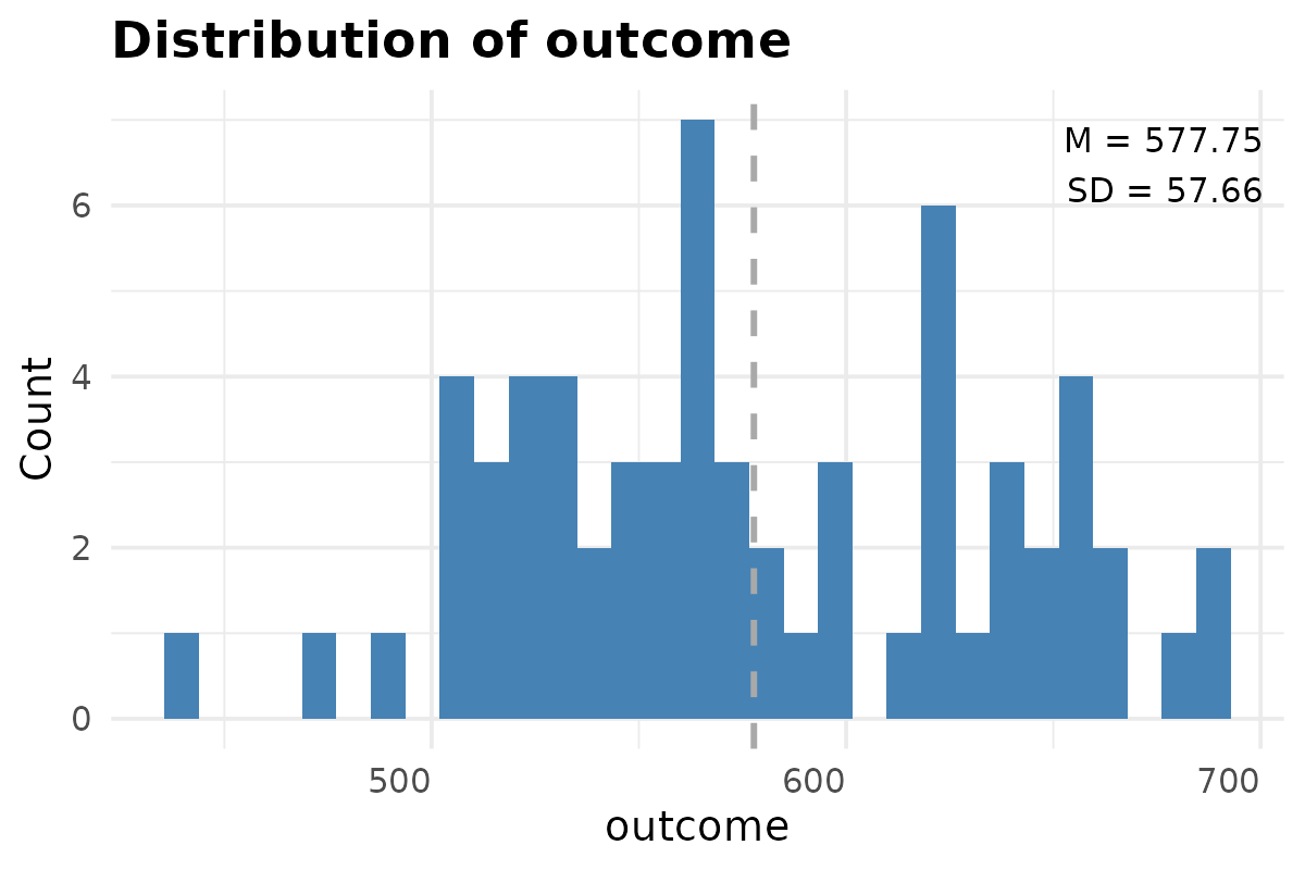
Additionally, I executed the ANOVA module in multiple parallel runs to quantify both the convergence variability of RMSE within each run (compared to the target values) and the variability of RMSE across runs (compared to the average simulated values).
result.parallel.aov <- parallel_aov(
                        parallel_start = 100,
                        return_best_solution = FALSE,
                        N = N,
                        levels =levels,
                        target_group_means = target_group_means,
                        target_f_list = target_f_vec,
                        factor_type = factor_type,
                        range = range,
                        formula = formula,
                        tolerance = 1e-8,
                        max_iter = 1e3,
                        init_temp = 1,
                        cooling_rate = NULL,
                        integer = FALSE,
                        checkGrim = FALSE,
                        max_step = .1,
                        min_decimals = 1)
I then plotted these RMSE distributions side-by-side to compare within versus between run variation.
plot_rmse(result.parallel.aov)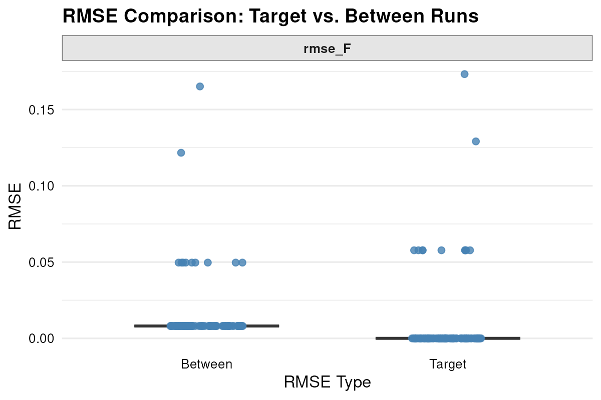 Note. The two clusters emerge due to the low decimal precision of the
reported F values. #
Note. The two clusters emerge due to the low decimal precision of the
reported F values. #
Descriptives and LM Module
In the replication attempt by Bardwell et al. (2007) patients with obstructive sleep apnea completed both fatigue and depression scales to examine whether mood symptoms or apnea severity better predict daytime fatigue [https://doi.org/10.1016/j.jad.2006.06.013]. The original study’s (Bardwell et al., 2003) raw data are not publicly available. Here, I apply the Descriptives and LM module of the DISCOURSE framework to simulate a synthetic dataset that reproduces their reported summary estimates.
Step 1.
I began by extracting the relevant descriptive parameters from the article.
N = 60
target_mean <- c(48.8, 17.3, 12.6, 10.8)
names(target_mean) <- c("Apnea.1", "Apnea.2", "Depression", "Fatigue")
target_sd <- c(27.1, 20.1, 11.3, 7.3)
integer = c(FALSE, FALSE, TRUE, TRUE)
range_matrix <- matrix(c(15, 0, 0, 0,
                         111, 80.9, 49, 28),
                       nrow = 2, byrow = TRUE)
I subsequently estimated the weights
weight.vec <- weights_vec(
  N = N,
  target_mean =  target_mean,
  target_sd =  target_sd,
  range = range_matrix,
  integer = integer
)
weight.vec
#> [[1]]
#> [1]  1.0000 33.6153
#>
#> [[2]]
#> [1]  1.0000 95.3409
#>
#> [[3]]
#> [1] 1.0000 4.6867
#>
#> [[4]]
#> [1] 1.0000 4.5158
and I ran the Descriptives module with default hyperparameters.
result.vec <- optim_vec(
N = N,
target_mean = target_mean,
target_sd = target_sd,
range = range_matrix,
integer = integer,
obj_weight = weight.vec,
tolerance = 1e-8,
max_iter = 1e5,
max_starts = 3,
init_temp = 1,
cooling_rate = NULL
)
#>
#> PSO is running...
#> Converged
#>
#>
#> PSO is running...
#> Converged
#>
#>
#> Mean 12.6 passed GRIM test. The mean is plausible.
#> | | | 0% | |= | 1% | |= | 2% | |== | 3% | |=== | 4% | |==== | 5% | |==== | 6% | |===== | 7% | |====== | 8% | |====== | 9% | |======= | 10% | |======== | 11% | |======== | 12% | |========= | 13% | |========== | 14% | |========== | 15% | |=========== | 16% | |============ | 17% | |============= | 18% | |============= | 19% | |============== | 20% | |=============== | 21% | |=============== | 22% | |================ | 23% | |================= | 24% | |================== | 25% | |================== | 26% | |=================== | 27% | |==================== | 28% | |==================== | 29% | |===================== | 30% | |====================== | 31% | |====================== | 32% | |======================= | 33% | |======================== | 34%
#> converged!
#>
#>
#> Mean 10.8 passed GRIM test. The mean is plausible.
#> | | | 0% | |= | 1% | |= | 2% | |== | 3% | |=== | 4% | |==== | 5% | |==== | 6% | |===== | 7% | |====== | 8% | |====== | 9% | |======= | 10% | |======== | 11% | |======== | 12% | |========= | 13% | |========== | 14% | |========== | 15% | |=========== | 16% | |============ | 17% | |============= | 18%
#> converged!The optimization converged exactly. Inspecting
summary(result.vec)
#> DISCOURSE Object Summary
#> -------------------------------------------------
#>
#> Achieved Loss of Optimization:
#>    Apnea.1    Apnea.2 Depression    Fatigue
#>          0          0          0          0
#>
#> RMSE of Summary Statistics
#>   Means:  0
#>   SDs:    0
#>
#> Means:
#>    Apnea.1    Apnea.2 Depression    Fatigue
#>   48.79311   17.26833   12.61667   10.75000
#>
#> SDs:
#>    Apnea.1    Apnea.2 Depression    Fatigue
#>  27.080425  20.121470  11.298855   7.308284
confirms that the simulated data reproduce the published means and SDs. I then visualized the error trajectories. For example, the error trajectory of the fatigue variable is:
plot_error(result.vec, run = 4)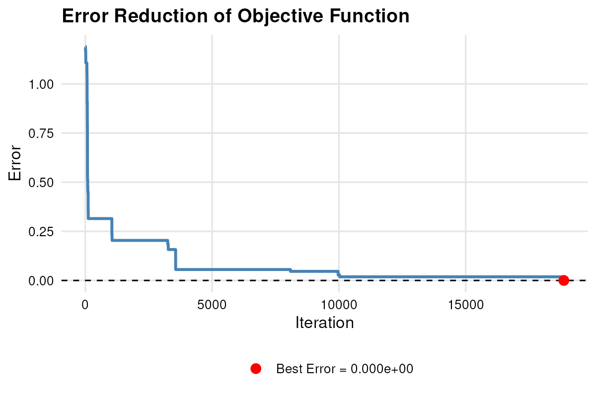
The estimated versus target descriptives are given by
plot_summary(result.vec, standardised = FALSE)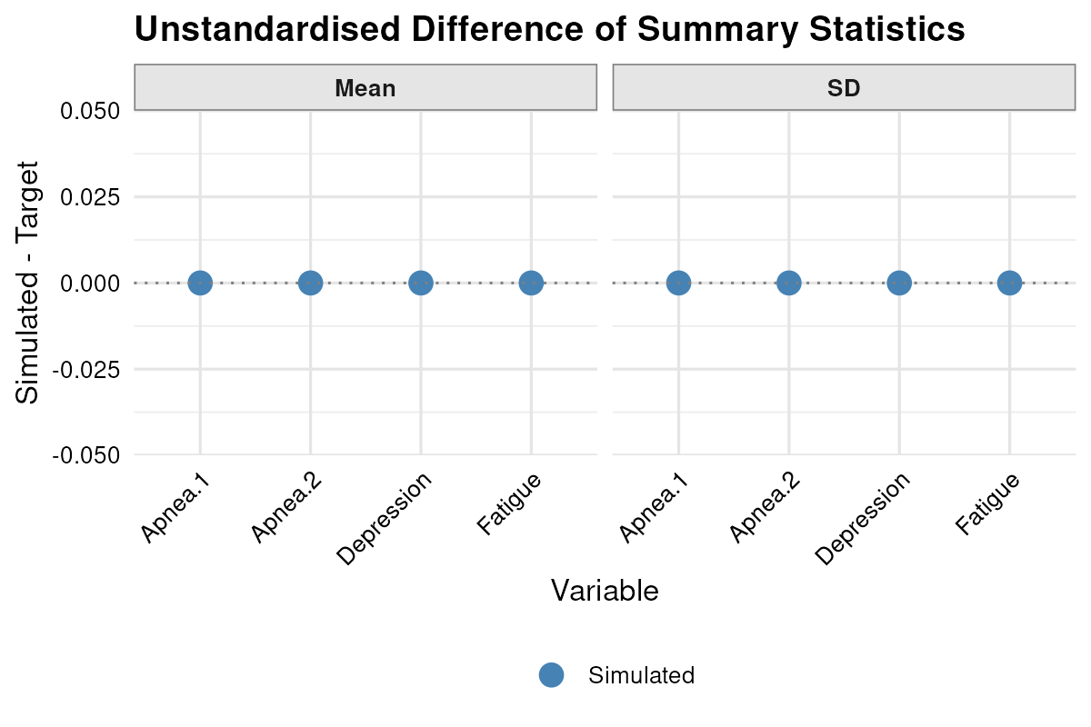
Finally, I saved the RMSE and relevant statistics,
get_rmse(result.vec)
#> $rmse_mean
#> [1] 0
#>
#> $rmse_sd
#> [1] 0
get_stats(result.vec)
#> $mean
#>    Apnea.1    Apnea.2 Depression    Fatigue
#>   48.79311   17.26833   12.61667   10.75000
#>
#> $sd
#>    Apnea.1    Apnea.2 Depression    Fatigue
#>  27.080425  20.121470  11.298855   7.308284
extracted the simulated dataset and inspected its distributions and frequencies.
data.vec <- result.vec$data
head(data.vec)
#>    Apnea.1   Apnea.2 Depression Fatigue
#> 1 43.80513  3.643460         12       1
#> 2 43.78154  4.375279         17      15
#> 3 25.49482 10.383827          6       5
#> 4 94.70739 22.410497          8       8
#> 5 46.20880 16.651429         14       2
#> 6 94.18734 11.846145          5       8
gridExtra::grid.arrange(grobs = plot_histogram(data.vec), ncol = 2)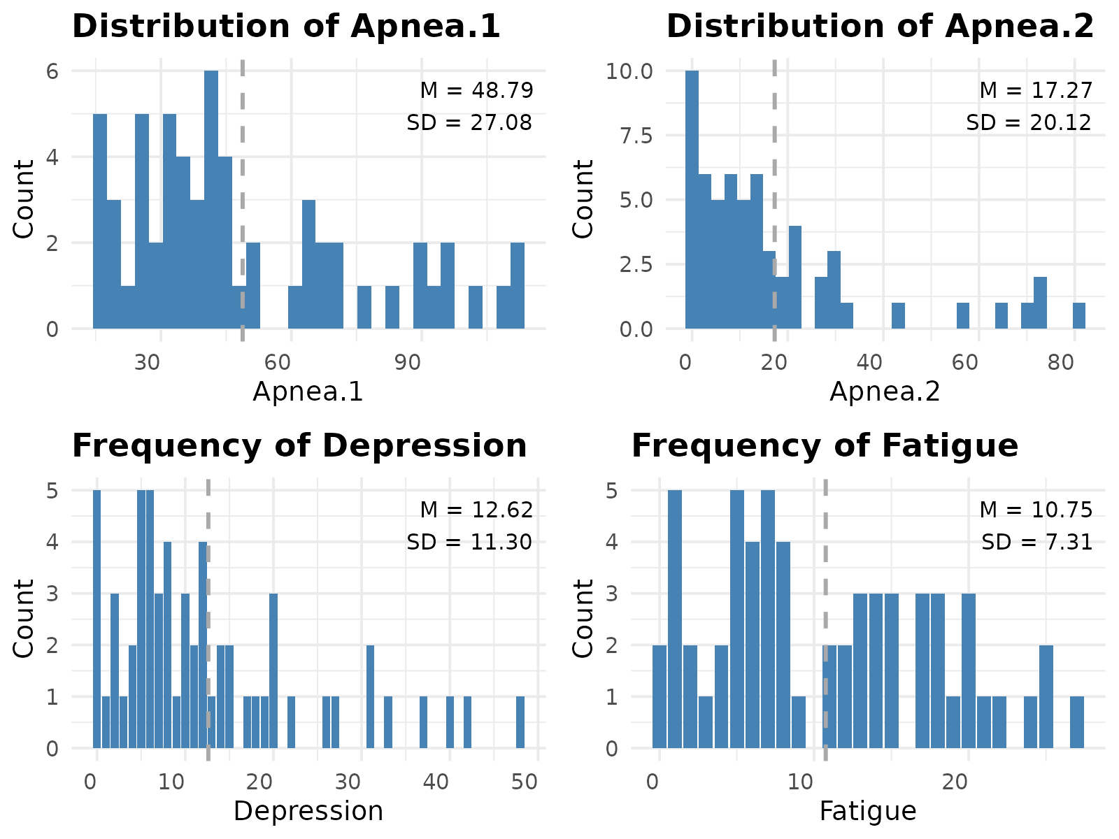
Step 2.
I began by extracting the relevant correlation and regression parameters from the article and handing off the simulated data from the Descriptives module for further use.
sim_data <- data.vec
target_reg <- c(4.020, 0.023, 0.008, 0.438)
names(target_reg) <- c("Apnea.1", "Apnea.2", "Depression", "Fatigue")
target_se <- c(NA, 0.034, 0.048, 0.066)
target_cor <-  c(NA, NA, NA, 0.11, 0.20, 0.68)
reg_equation <- "Fatigue ~ Apnea.1 + Apnea.2 + Depression"
I subsequently estimated the weights
result.weight.lm <- weights_est(
module = "lm",
sim_runs = 1,
sim_data = sim_data,
reg_equation = reg_equation,
target_cor = target_cor,
target_reg = target_reg,
target_se = target_se,
tol = 1e-8,
max_iter = 1e5,
init_temp = 1,
cooling_rate = NULL
)
#> | | | 0% | |= | 1% | |= | 2% | |== | 3% | |=== | 4% | |==== | 5% | |==== | 6% | |===== | 7% | |====== | 8% | |====== | 9% | |======= | 10% | |======== | 11% | |======== | 12% | |========= | 13% | |========== | 14% | |========== | 15% | |=========== | 16% | |============ | 17% | |============= | 18% | |============= | 19% | |============== | 20% | |=============== | 21% | |=============== | 22% | |================ | 23% | |================= | 24% | |================== | 25% | |================== | 26% | |=================== | 27% | |==================== | 28% | |==================== | 29% | |===================== | 30% | |====================== | 31% | |====================== | 32% | |======================= | 33% | |======================== | 34% | |======================== | 35% | |========================= | 36% | |========================== | 37% | |=========================== | 38% | |=========================== | 39% | |============================ | 40% | |============================= | 41% | |============================= | 42% | |============================== | 43% | |=============================== | 44% | |================================ | 45% | |================================ | 46% | |================================= | 47% | |================================== | 48% | |================================== | 49% | |=================================== | 50% | |==================================== | 51% | |==================================== | 52% | |===================================== | 53% | |====================================== | 54% | |====================================== | 55% | |======================================= | 56% | |======================================== | 57% | |========================================= | 58% | |========================================= | 59% | |========================================== | 60% | |=========================================== | 61% | |=========================================== | 62% | |============================================ | 63% | |============================================= | 64% | |============================================== | 65% | |============================================== | 66% | |=============================================== | 67% | |================================================ | 68% | |================================================ | 69% | |================================================= | 70% | |================================================== | 71% | |================================================== | 72% | |=================================================== | 73% | |==================================================== | 74% | |==================================================== | 75% | |===================================================== | 76% | |====================================================== | 77% | |======================================================= | 78% | |======================================================= | 79% | |======================================================== | 80% | |========================================================= | 81% | |========================================================= | 82% | |========================================================== | 83% | |=========================================================== | 84% | |============================================================ | 85% | |============================================================ | 86% | |============================================================= | 87% | |============================================================== | 88% | |============================================================== | 89% | |=============================================================== | 90% | |================================================================ | 91% | |================================================================ | 92% | |================================================================= | 93% | |================================================================== | 94% | |================================================================== | 95% | |=================================================================== | 96% | |==================================================================== | 97% | |===================================================================== | 98% | |===================================================================== | 99% | |======================================================================| 100%
#> Best error in start 1 is 0.003927922
#>
#> The estimated weights are: 1 1.83
weight.lm <- result.weight.lm$weights
weight.lm
#> [1] 1.00 1.83and I ran the LM module with default hyperparameters.
result.lm <- optim_lm(
sim_data = sim_data,
reg_equation = reg_equation,
target_cor = target_cor,
target_reg = target_reg,
target_se = target_se,
weight = weight.lm,
tol = 1e-8,
max_iter = 1e5,
max_starts = 1,
init_temp = 1,
cooling_rate = NULL
)
#> | | | 0% | |= | 1% | |= | 2% | |== | 3% | |=== | 4% | |==== | 5% | |==== | 6% | |===== | 7% | |====== | 8% | |====== | 9% | |======= | 10% | |======== | 11% | |======== | 12% | |========= | 13% | |========== | 14% | |========== | 15% | |=========== | 16% | |============ | 17% | |============= | 18% | |============= | 19% | |============== | 20% | |=============== | 21% | |=============== | 22% | |================ | 23% | |================= | 24% | |================== | 25% | |================== | 26% | |=================== | 27% | |==================== | 28% | |==================== | 29% | |===================== | 30% | |====================== | 31% | |====================== | 32% | |======================= | 33% | |======================== | 34% | |======================== | 35% | |========================= | 36% | |========================== | 37% | |=========================== | 38% | |=========================== | 39% | |============================ | 40% | |============================= | 41% | |============================= | 42% | |============================== | 43% | |=============================== | 44% | |================================ | 45% | |================================ | 46% | |================================= | 47% | |================================== | 48% | |================================== | 49% | |=================================== | 50% | |==================================== | 51% | |==================================== | 52% | |===================================== | 53% | |====================================== | 54% | |====================================== | 55% | |======================================= | 56% | |======================================== | 57% | |========================================= | 58% | |========================================= | 59% | |========================================== | 60% | |=========================================== | 61% | |=========================================== | 62% | |============================================ | 63% | |============================================= | 64% | |============================================== | 65% | |============================================== | 66% | |=============================================== | 67% | |================================================ | 68% | |================================================ | 69% | |================================================= | 70% | |================================================== | 71% | |================================================== | 72% | |=================================================== | 73% | |==================================================== | 74% | |==================================================== | 75% | |===================================================== | 76% | |====================================================== | 77% | |======================================================= | 78% | |======================================================= | 79% | |======================================================== | 80% | |========================================================= | 81% | |========================================================= | 82% | |========================================================== | 83% | |=========================================================== | 84% | |============================================================ | 85% | |============================================================ | 86% | |============================================================= | 87% | |============================================================== | 88% | |============================================================== | 89% | |=============================================================== | 90% | |================================================================ | 91% | |================================================================ | 92% | |================================================================= | 93% | |================================================================== | 94% | |================================================================== | 95% | |=================================================================== | 96% | |==================================================================== | 97% | |===================================================================== | 98% | |===================================================================== | 99% | |======================================================================| 100%
#> Best error in start 1 is 0.009305535The optimization converged with reaching Max Iterations and a low RMSE. Inspecting
summary(result.lm)
#> DISCOURSE Object Summary
#> -------------------------------------------------
#>
#> Achieved Loss of Optimization:  0.009305535
#>
#> RMSE of Summary Statistics
#>   Correlations:             0
#>   Regression Coefficients:  0.001581139
#>   Standard Errors:          0.007549834
#>
#> Regression Model:
#> "Fatigue ~ Apnea.1 + Apnea.2 + Depression"
#>
#> Simulated Data Summary:
#>   Coefficients:
#> (Intercept)     Apnea.1     Apnea.2  Depression
#> 4.017945944 0.021949213 0.009467089 0.435741307
#>
#>   Std. Errors:
#> (Intercept)     Apnea.1     Apnea.2  Depression
#>  1.65390076  0.02651084  0.03675280  0.06460915
#>
#>   Correlations:
#> [1] 0.16332180 0.03386227 0.24214044 0.10840058 0.20247134 0.68273634
#>
#>   Means:
#>    Apnea.1    Apnea.2 Depression    Fatigue
#>   48.79311   17.26833   12.61667   10.75000
#>
#>   SDs:
#>    Apnea.1    Apnea.2 Depression    Fatigue
#>  27.080425  20.121470  11.298855   7.308284
confirms that the simulated data closely reproduce the published regression and correlation parameters. I then visualized the error,
plot_error(result.lm)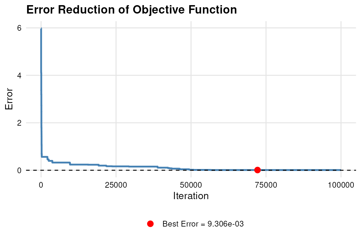 the error-ratio trajectories,
plot_error_ratio(result.lm)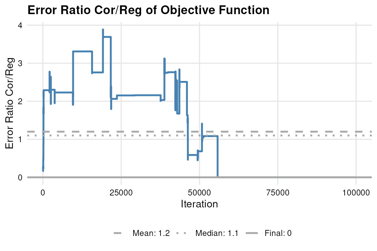 and illustrated the estimated versus target descriptives with
plot_summary(result.lm, standardised = FALSE)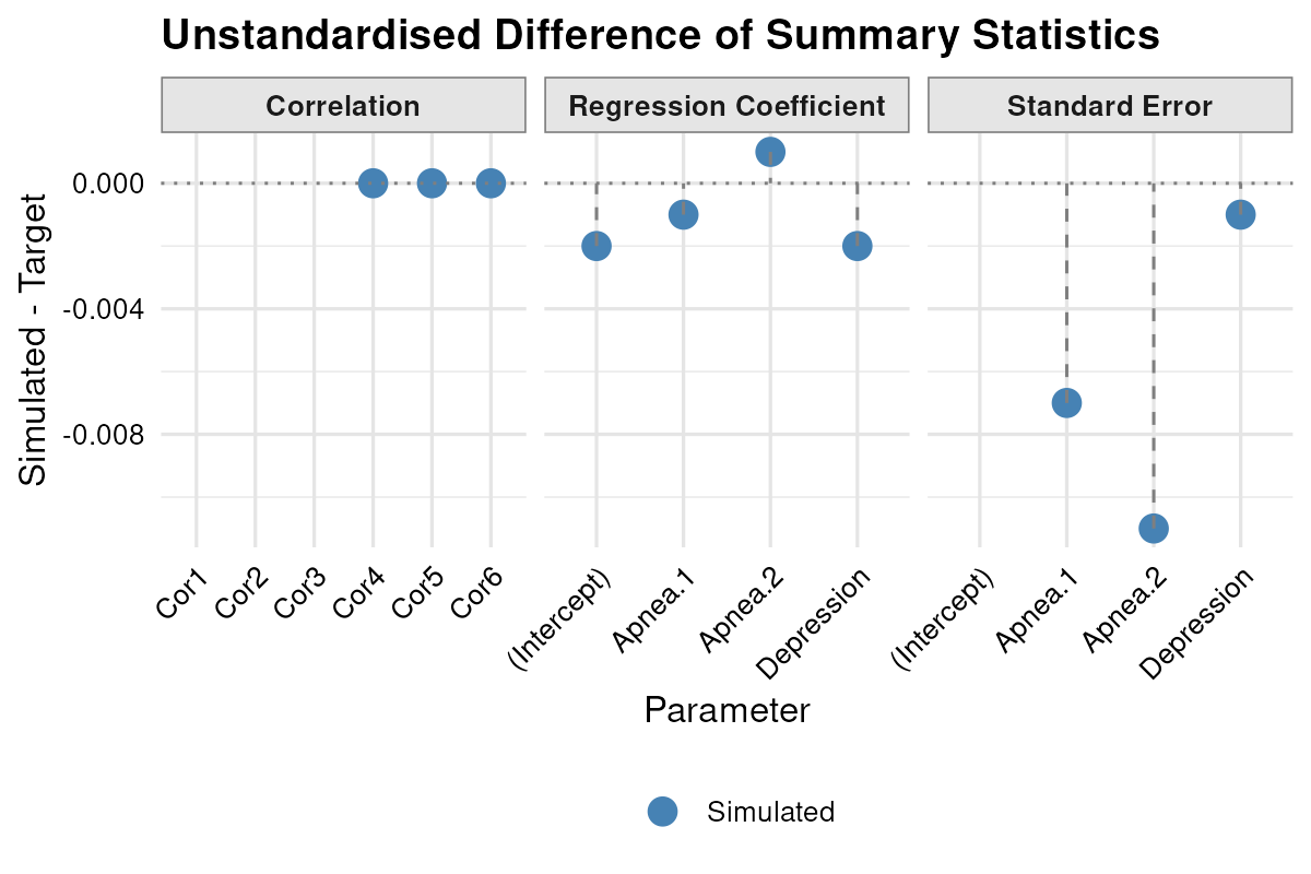
Finally, I saved the RMSE and relevant statistics,
get_rmse(result.lm)
#> $rmse_cor
#> [1] 0
#>
#> $rmse_reg
#> [1] 0.001581139
#>
#> $rmse_se
#> [1] 0.007549834
get_stats(result.lm)
#> $model
#>
#> Call:
#> stats::lm(formula = eq, data = data_df)
#>
#> Coefficients:
#> (Intercept)      Apnea.1      Apnea.2   Depression
#>    4.017946     0.021949     0.009467     0.435741
#>
#>
#> $reg
#> (Intercept)     Apnea.1     Apnea.2  Depression
#> 4.017945944 0.021949213 0.009467089 0.435741307
#>
#> $se
#> (Intercept)     Apnea.1     Apnea.2  Depression
#>  1.65390076  0.02651084  0.03675280  0.06460915
#>
#> $cor
#> [1] 0.16332180 0.03386227 0.24214044 0.10840058 0.20247134 0.68273634
#>
#> $mean
#>    Apnea.1    Apnea.2 Depression    Fatigue
#>   48.79311   17.26833   12.61667   10.75000
#>
#> $sd
#>    Apnea.1    Apnea.2 Depression    Fatigue
#>  27.080425  20.121470  11.298855   7.308284
extracted the simulated dataset and inspected its partial regression plots.
data.lm <- result.lm$data
head(data.lm)
#>     Apnea.1   Apnea.2 Depression Fatigue
#> 1  15.58191  8.059517         18       1
#> 2 103.63091 26.795559          7      15
#> 3  17.09136  7.660308          0       5
#> 4  39.89401 20.600598         10       8
#> 5  94.18734  4.670536          6       2
#> 6  25.49482 12.985366          7       8
partial.plots <- plot_partial_regression(lm(reg_equation, data.lm))
gridExtra::grid.arrange(grobs = partial.plots, ncol = 2)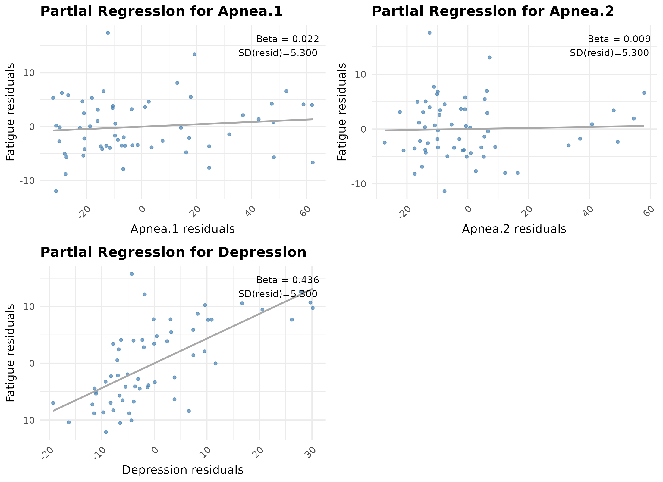
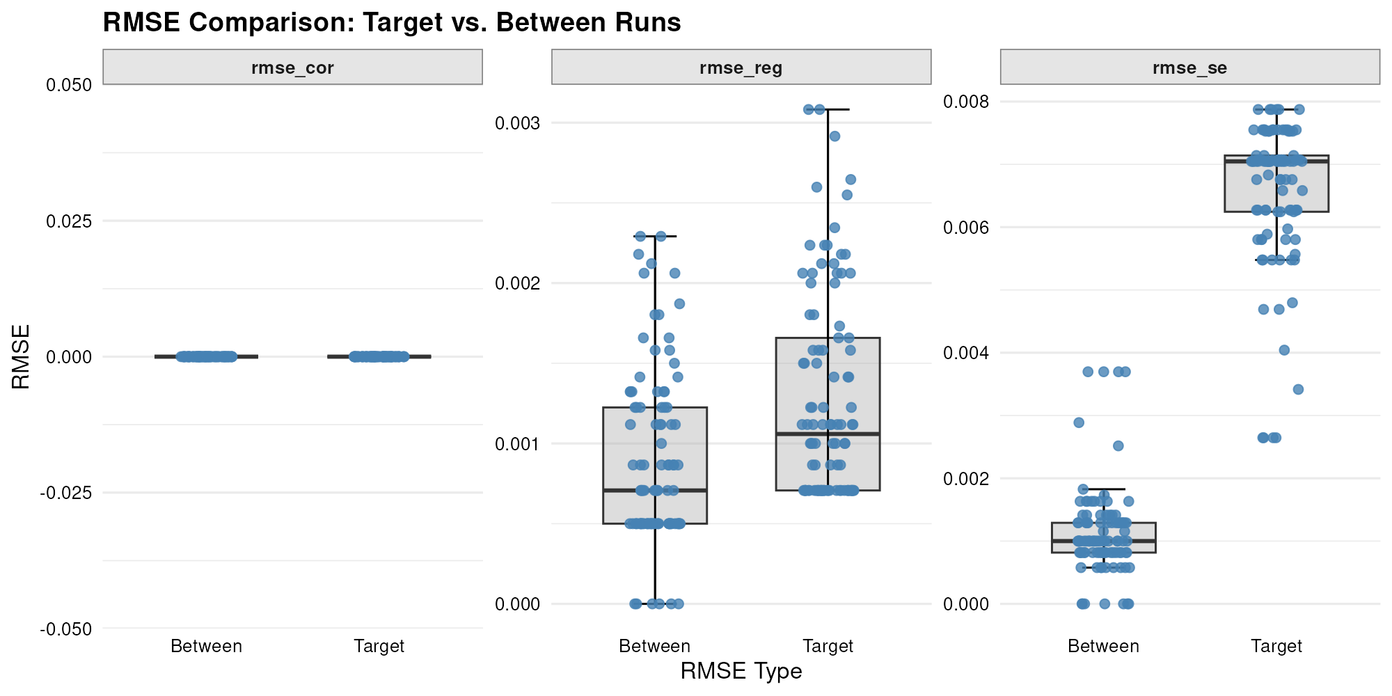
Additionally, I executed the LM module in multiple parallel runs to quantify both the convergence variability of RMSE within each run (compared to the target values) and the variability of RMSE across runs (compared to the average simulated values).
result.parallel.lm <- parallel_lm(
  parallel_start = 100,
  return_best_solution = FALSE,
  sim_data = sim_data,
  reg_equation = reg_equation,
  target_cor = target_cor,
  target_reg = target_reg,
  target_se = target_se,
  weight = weight.lm,
  tol = 1e-8,
  max_iter = 1e5,
  max_starts = 1,
  init_temp = 1,
  cooling_rate = NULL
)
I then plotted these RMSE distributions side-by-side to compare within versus between run variation.
plot_rmse(result.parallel.lm)